Jupyter Notebooks
Python Jupyter notebooks are an excellent way to experiment with data science and visualization. Using the higlass-jupyter extension, you can use HiGlass directly from within a Jupyter notebook.
Installation
To use higlass within a Jupyter notebook you need to install a few packages and enable the jupyter extension:
pip install jupyter hgflask higlass-jupyter

jupyter nbextension install --py --sys-prefix --symlink higlass_jupyter
jupyter nbextension enable --py --sys-prefix higlass_jupyter
Uninstalling
jupyter nbextension uninstall --py --sys-prefix higlass_jupyter
Usage
To instantiate a HiGlass component within a Jupyter notebook, we first need
to specify which data should be loaded. This can be accomplished with the
help of the hgflask.client module:
import higlass_jupyter as hiju
import hgflask.client as hgc

conf = hgc.ViewConf([
    hgc.View([
        hgc.Track(track_type='top-axis', position='top'),
        hgc.Track(track_type='heatmap', position='center',
                 tileset_uuid='CQMd6V_cRw6iCI_-Unl3PQ',
                  api_url="http://higlass.io/api/v1/",
                  height=250,
                 options={ 'valueScaleMax': 0.5 }),

    ])
])

hiju.HiGlassDisplay(viewconf=conf.to_json())
The result is a fully interactive HiGlass view direcly embedded in the Jupyter notebook.
Serving local data
To view local data, we need to define the tilesets and set up a temporary server.
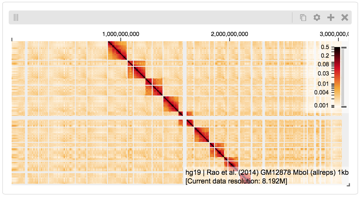
Cooler Files
Creating the server:
import hgflask.tilesets as hfti
import hgflask.server as hgse

ts = hfti.cooler(
    '../data/Dixon2012-J1-NcoI-R1-filtered.100kb.multires.cool')

server = hgse.start(tilesets=[ts])
And displaying the dataset in the client:
import higlass_jupyter as hiju
import hgflask.client as hgc

conf = hgc.ViewConf([
    hgc.View([
        hgc.Track(track_type='top-axis', position='top'),
        hgc.Track(track_type='heatmap', position='center',
                 tileset_uuid=ts.uuid,
                  api_url=server.api_address,
                  height=250
                 options={ 'valueScaleMax': 0.5 }),

    ])
])

hiju.HiGlassDisplay(viewconf=conf.to_json())
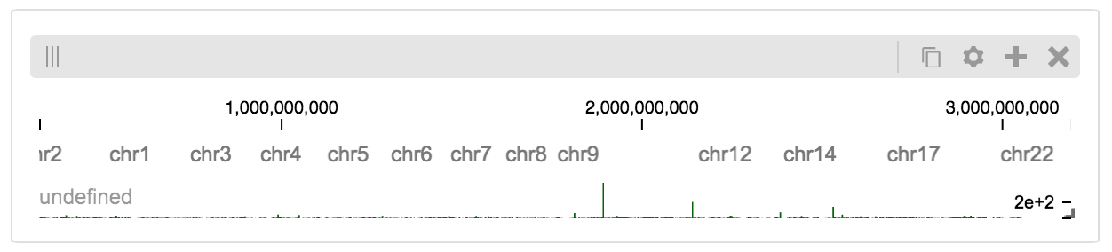
BigWig Files
In this example, we’ll set up a server containing both a chromosome labels track and a bigwig track. Furthermore, the bigwig track will be ordered according to the chromosome info in the specified file.
import hgtiles.chromsizes as hgch

import hgflask.server as hgse
import hgflask.tilesets as hfti


chromsizes_fp = '../data/chromSizes_hg19_reordered.tsv'
bigwig_fp = '../data/wgEncodeCaltechRnaSeqHuvecR1x75dTh1014IlnaPlusSignalRep2.bigWig'

chromsizes = hgch.get_tsv_chromsizes(chromsizes_fp)

ts_r = hfti.bigwig(bigwig_fp, chromsizes=chromsizes)
cs_r = hfti.chromsizes(chromsizes_fp)

server = hgse.start(tilesets=[ts_r, cs_r])
The client view will be composed such that three tracks are visible. Two of them are served from the local server.
import higlass_jupyter as hiju
import hgflask.client as hgc

conf = hgc.ViewConf([
    hgc.View([
        hgc.Track(track_type='top-axis', position='top'),

        hgc.Track(track_type='horizontal-chromosome-labels', position='top',
                 tileset_uuid=cs_r.uuid, api_url=server.api_address),
        hgc.Track(track_type='horizontal-bar', position='top',
                  tileset_uuid=ts_r.uuid, api_url=server.api_address,
                 options={ 'height': 40 }),
    ])
])

hiju.HiGlassDisplay(viewconf=conf.to_json())
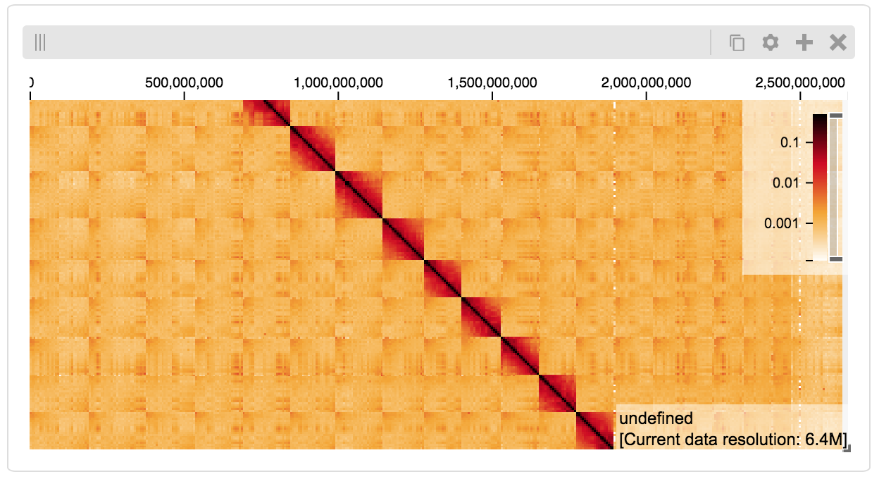
Serving custom data
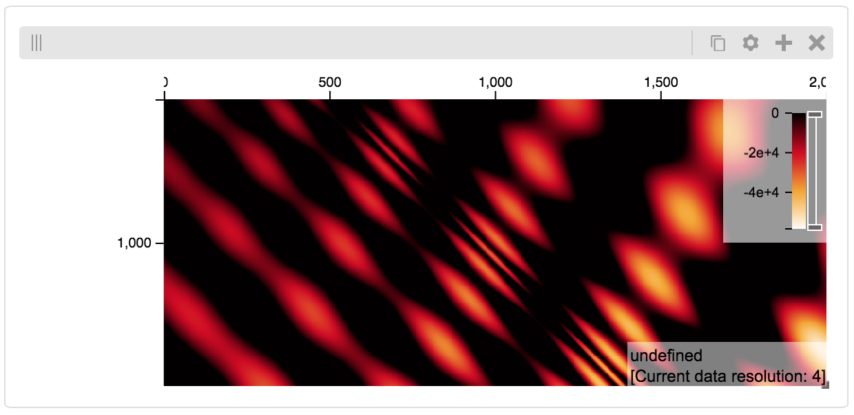
We can also explore a numpy matrix. To start let’s make the matrix using the Eggholder function.
import math
import numpy as np
import itertools as it

dim = 2000

data = np.zeros((dim, dim))
for x,y in it.product(range(dim), repeat=2):
    data[x][y] = (-(y + 47) * math.sin(math.sqrt(abs(x / 2 + (y+47))))
                             - x * math.sin(math.sqrt(abs(x - (y+47)))))
Then we can define the data and tell the server how to render it.
import functools as ft
import hgtiles.npmatrix as hgnp

import hgflask.server as hgse
import hgflask.tilesets as hfti

ts = hfti.Tileset(
    tileset_info=lambda: hgnp.tileset_info(data),
    tiles=lambda tids: hgnp.tiles_wrapper(data, tids)
)

server = hgse.start([ts])
Finally, we create the HiGlass component which renders it, along with axis labels:
import higlass_jupyter as hiju
import hgflask.client as hgc

conf = hgc.ViewConf([
    hgc.View([
        hgc.Track(track_type='top-axis', position='top'),
        hgc.Track(track_type='left-axis', position='left'),
        hgc.Track(track_type='heatmap', position='center',
                 tileset_uuid=ts.uuid,
                  api_url=server.api_address,
                  height=250,
                 options={ 'valueScaleMax': 0.5 }),

    ])
])

hiju.HiGlassDisplay(viewconf=conf.to_json())
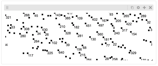
Displaying Many Points
To display, for example, a list of 1 million points in a HiGlass window inside of a Jupyter notebook. First we need to import the custom track type for displaying labelled points:
%%javascript

require(["https://unpkg.com/higlass-labelled-points-track@0.1.7/dist/higlass-labelled-points-track"],
    function(hglib) {

});
Then we have to set up a data server to output the data in “tiles”.
import hgtiles.points as hgpo
import hgtiles.utils as hgut

import hgflask.server as hfse
import hgflask.tilesets as hfti

import numpy as np
import pandas as pd

length = int(1e6)
df = pd.DataFrame({
    'x': np.random.random((length,)),
    'y': np.random.random((length,)),
    'v': range(1, length+1),
})

# get the tileset info (bounds and such) of the dataset
tsinfo = hgpo.tileset_info(df, 'x', 'y')

ts = hfti.Tileset(
    tileset_info=lambda: tsinfo,
    tiles=lambda tile_ids: hgpo.format_data(
                hgut.bundled_tiles_wrapper_2d(tile_ids,
                    lambda z,x,y,width=1,height=1: hgpo.tiles(df, 'x', 'y',
                        tsinfo, z, x, y, width, height))))

# start the server
server = hfse.start([ts])
And finally, we can create a HiGlass client in the browser to view the data:
import hgflask.client as hfc
import higlass_jupyter as hiju

hgc = hfc.ViewConf([
    hfc.View([
        hfc.Track(
            track_type='labelled-points-track',
            position='center',
            tileset_uuid=ts.uuid,
            api_url=server.api_address,
            height=200,
            options={
                'labelField': 'v'
            })
    ])
])

hiju.HiGlassDisplay(viewconf=hgc.to_json())